Like we know the answer, we know that a laptop cannot be that powerful to have such capability, that it handles million users, but it was always vague to me and I did not know the exact technical reason why it is the case. Where things break? Where are the bottlenecks? Are they related to hardware or something else? Is this a framework dependent question? Or what actually stops us from going there.
This will be a deep dive on why my device cannot handle that many users, not just relying on the answer of “we need a big machine for many users”, but instead to actually understand when we need to pull the levers to reach that many users.
Low level understanding of request cycle
To understand where things break at scale, we first need to understand what actually happens when a request comes in, you hit http://localhost:3000/users/42 and get a JSON response in 5ms locally. Let’s unfold it, because the cracks that appear at 1M users are sitting right here, invisible.
(We’ll be looking at this from a Linux kernel perspective since most servers run Linux but my project is in .NET, so metrics and performance numbers will be from the Windows ecosystem. Don’t mind the mix.)
When your server starts, it makes a system call socket() asking the OS kernel for a socket. A socket is just a kernel-managed data structure: a buffer for incoming bytes, a buffer for outgoing bytes, and some metadata. The process then calls bind() to claim port 3000, and listen() to tell the kernel: _“when SYN packets arrive on this port, queue them.”
At this point, your process isn’t handling connections the kernel is. Your process is sleeping, blocked on an accept() call. The kernel maintains two queues here: the SYN queue (incoming connection requests) and the accept queue (connections that have completed the TCP handshake and are waiting for your app to pick them up). Once your app calls accept(), it pulls a connection off that queue and gets to work.
From there, the kernel’s send and receive buffers handle the actual bytes, incoming request bytes land in the receive buffer, and your response bytes go out through the send buffer. These are separate from accept and request queue.
Your app then parses those bytes into a request object, maps it to a handler, and if there’s a database call involved, opens another TCP connection this time to Postgres. Postgres does its thing, returns rows. Your app serializes them to JSON. More CPU work. Finally, the app calls write() on the file descriptor, the kernel copies the bytes into the socket’s send buffer, and they go out on the wire.
Now where things break?
Layer 1: 0 → 100 concurrent users the first honest bottleneck
Your laptop can absolutely handle 100 concurrent users. But how you’re handling them starts to matter.
Model A: One Thread Per Connection
Threads share memory, so they’re cheaper ~1–2MB stack per thread.
Why this breaks?
- Context switches. Every time the OS scheduler swaps from one thread to another, it has to save the current thread’s CPU registers (general-purpose, floating-point, vector roughly 15+ registers), update scheduler bookkeeping, and load the next thread’s registers. The raw switch itself takes ~1–5 microseconds.
That doesn’t sound like much, but if you have 10,000 threads and the scheduler round-robins through them, you’re burning tens of milliseconds of pure overhead per full cycle not counting the cache-miss penalty afterward, which can extend the effective cost to 10–50 microseconds per switch. You’re now spending more CPU on switching than on doing actual work.
-
CPU cache thrashing. Every context switch cools the cache the new thread’s data isn’t there. Cache misses turn a 1ns operation into 100ns. At high thread counts, your CPU spends most of its time waiting for memory, not computing.
-
Memory. 2MB stack × 10,000 threads = 20GB RAM just for thread stacks. Possible, but not practical though to be fair, this is lazily committed, starting from 4KB and doubling at each threshold up to 2MB, so it’s not 20GB all at once.
But the deeper reason this model is wrong and this is the insight that led to async/event-loop architectures is that most of those threads aren’t doing anything. They’re blocked on I/O. Waiting for the database. Waiting for the network. Each thread is holding 2MB of stack and a kernel scheduler slot just to wait.
Model B: One Thread, Non-Blocking I/O, Event Loop (Node.js, async Python)
Instead of blocking a thread on each I/O operation, we tell the kernel: “let me know when any of these 10,000 sockets has data ready.” The kernel checks which sockets are ready and alerts the server → server handles them → they either finish or go to I/O operation → repeat.
Because I/O is the slow part, a single CPU thread can juggle thousands of connections as long as each handler does only a tiny amount of CPU work between I/O calls.
The kernel maintains the watched file descriptors as a persistent data structure. When an FD becomes ready, it gets put on a ready list and your event loop picks it up.
Model C: Thread Pool with Completion-Based Async I/O (.NET, Java virtual threads, Go)
Many OS threads, but threads aren’t tied to specific connections. When a request awaits I/O, its thread is released back to the pool and picks up other work. When the I/O completes, any available thread resumes the continuation.
This gives you Node’s I/O efficiency and real CPU parallelism across cores.
Layer 2 : 100 → 1000 concurrent users where the cracks first appear
There is less chance our PC will break here for handling requests, but here are certain things to consider.
Accept queue overflow
The two kernel queues from earlier the SYN queue (half-open connections during handshake) and the accept queue (established connections waiting for your app to call accept()). At this scale, the accept queue is the one that breaks first.
Your app is slow to call accept() because it’s busy serving existing requests. The accept queue fills. New clients experience connection failures but your monitoring on existing requests looks fine. You see occasional “connection refused” errors. This is called accept queue overflow.
File descriptors
These are a Linux concept. Windows uses HANDLEs instead same idea (kernel-tracked references to open resources), different implementation. We’ll focus on Linux since most servers run there.
When your process calls socket(), accept(), or open(), the kernel creates an entry in a per-process table called the file descriptor table. The “file descriptor” you get back (an integer like 5 or 247) is just an index into this table. The actual entry points to a kernel structure (struct file in Linux) which holds the socket buffers, the connection state, the read/write position, permissions, and so on.
The kernel doesn’t let a single process hold unlimited FDs for two reasons:
The table is bounded per-process. Linux traditionally defaults to a soft limit of 1024 FDs per process, though modern distros often raise this for services. You can check with ulimit -n and raise it via ulimit or systemd unit files.
This isn’t because the kernel can’t handle more it absolutely can it’s a guardrail. The per-process limit isolates one buggy process from taking resources others need. A separate system-wide limit (fs.file-max) protects total kernel memory from being exhausted by all processes combined. A runaway process leaking sockets hits its per-process limit first, before it can hurt the rest of the machine.
Why FD accounting matters?
A single incoming HTTP request in a typical app touches multiple FDs:
- 1 FD for the client socket (per request)
- 1 FD for the database connection but borrowed from a pool, not opened per request. A pool of 20 connections means 20 FDs total for DB, regardless of how many requests are flowing through.
- 1 FD per downstream microservice call (also typically pooled via HttpClient/keep-alive)
- 1 FD per file you open to read/write
- 1 FD per Redis connection (also pooled)
Without pooling, 1000 concurrent requests × 5 backends = 5000 FDs. With pooling, it’s more like 1000 client FDs + ~100 pooled backend FDs = 1100 total. Pooling is what keeps FD counts manageable at scale and is the reason real production apps don’t blow through their FD limits even under heavy load.
With those limits in mind, here’s what actually happens.
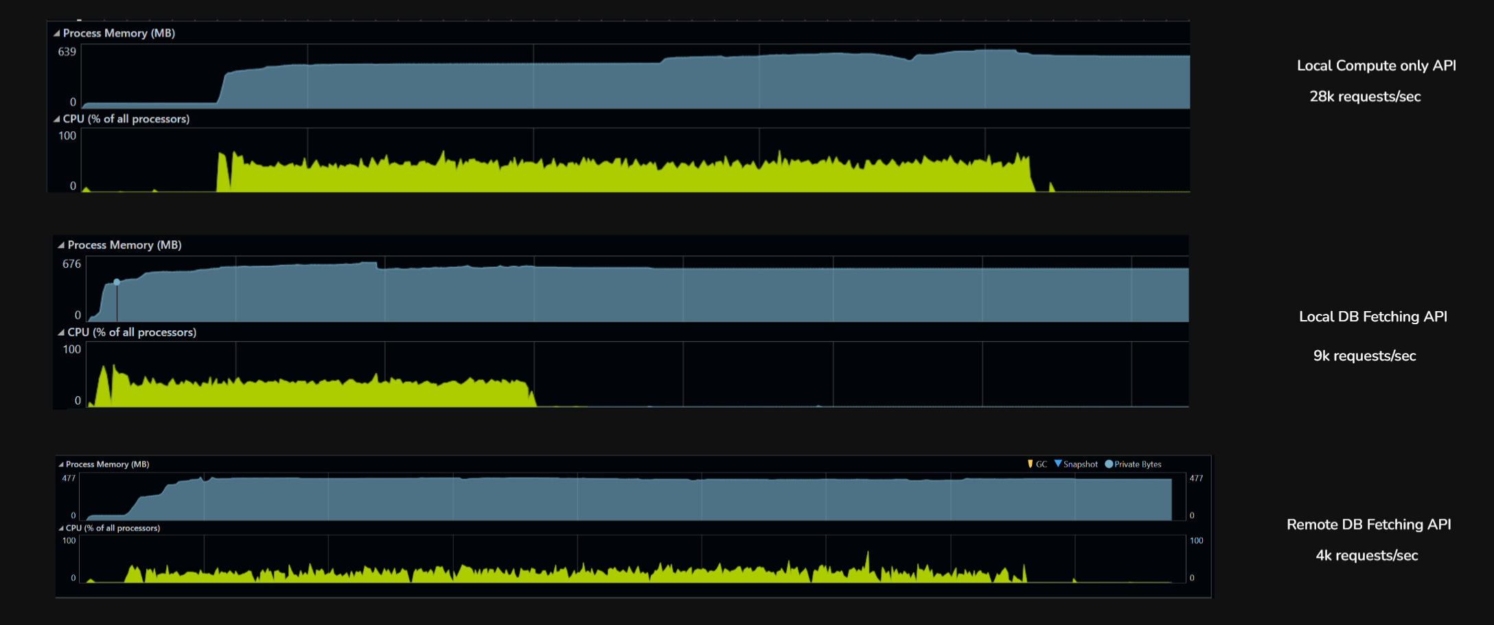
I’m starting at 1000 virtual users at the system. The setup has two .NET APIs one is compute-only, it calculates age when you pass a birthdate. The other hits Postgres, fetching a value by key. The database has integer keys between 1 and 1000, each mapped to a random GUID, and that’s what the API returns.
Database is configured at 200 max connections. Load is generated with k6, the .NET APIs are running under a profiler, and the machine is 16GB RAM, 8-core CPU.
Testing with 1000 virtual users
We are testing it in 3 scenarios to see what are the bottlenecks we will enounter,
- Local Date Api, Just compute only everything is local the client and server, this is to see the capability of CPU and memory
- Local Fetch Api with Database call: this is to see what happens when DB is involved
- Remote Fetch Api with Database call: this is to see when network is involved
| Metric | Local, no DB (GetAge) |
Local, with DB (FetchUUID) |
Remote, with DB (FetchUUID) |
|---|---|---|---|
| Throughput (rps) | 28,807 | 9,326 | 4,584 |
| Total requests (6 min) | 10,370,595 | 3,357,423 | 1,650,602 |
| p50 latency | 19 ms | 53 ms | 123 ms |
| p95 latency | 35 ms | 113 ms | 251 ms |
| p99 latency | 50 ms | 296 ms | ~310 ms |
| Max latency | 2.3 s | 15.7 s | 5.7 s |
| Failures | 0 | 55 (0.002%) | 2 (0.0001%) |
| Bottleneck | Kernel + Kestrel | Postgres + connection pool | Wi-Fi network |
Local, no DB (28,807 rps). k6 and the .NET app on the same machine, endpoint does pure CPU work (date math). Nothing to wait on. The only limit is how fast the kernel can shovel HTTP requests through Kestrel. Latency is tight (p50 to p99 spread is only 2.5x), almost no tail. This is the server’s true ceiling when nothing external is in the way.
Local, with DB (9,326 rps). Same setup, but the endpoint now hits Postgres for every request. Throughput drops 3x because each request now waits on a connection from the pool, executes SQL, and parses a row. The 15.7-second max latency is requests stuck in the connection pool queue when all 200 connections are busy. The bottleneck moved from the kernel to the database stack.
Remote, with DB (4,584 rps). Same DB endpoint, but k6 now runs on a separate laptop hitting the server over Wi-Fi. Throughput drops another 2x but the DB is no longer the bottleneck. The network is. Median latency jumps to 123ms (almost entirely Wi-Fi round-trip), and the server sits idle most of the time waiting for the next packet. The DB stack could handle far more load; the network just won’t deliver it.
The three runs show how performance bottlenecks are layered and how each one hides the next. On localhost with no I/O, the server hit its true CPU ceiling at 28K rps. Add a database call, and the ceiling drops to 9K rps because the connection pool and Postgres become the slowest link. Move the client across a Wi-Fi network, and the ceiling drops again to 4.5K rps but now the database isn’t the bottleneck anymore, the network is. The same DB code that looked like the problem in run two is invisible in run three, because something even slower sits in front of it. This concludes: optimizing any layer is pointless until we haven’t identified the bottleneck.
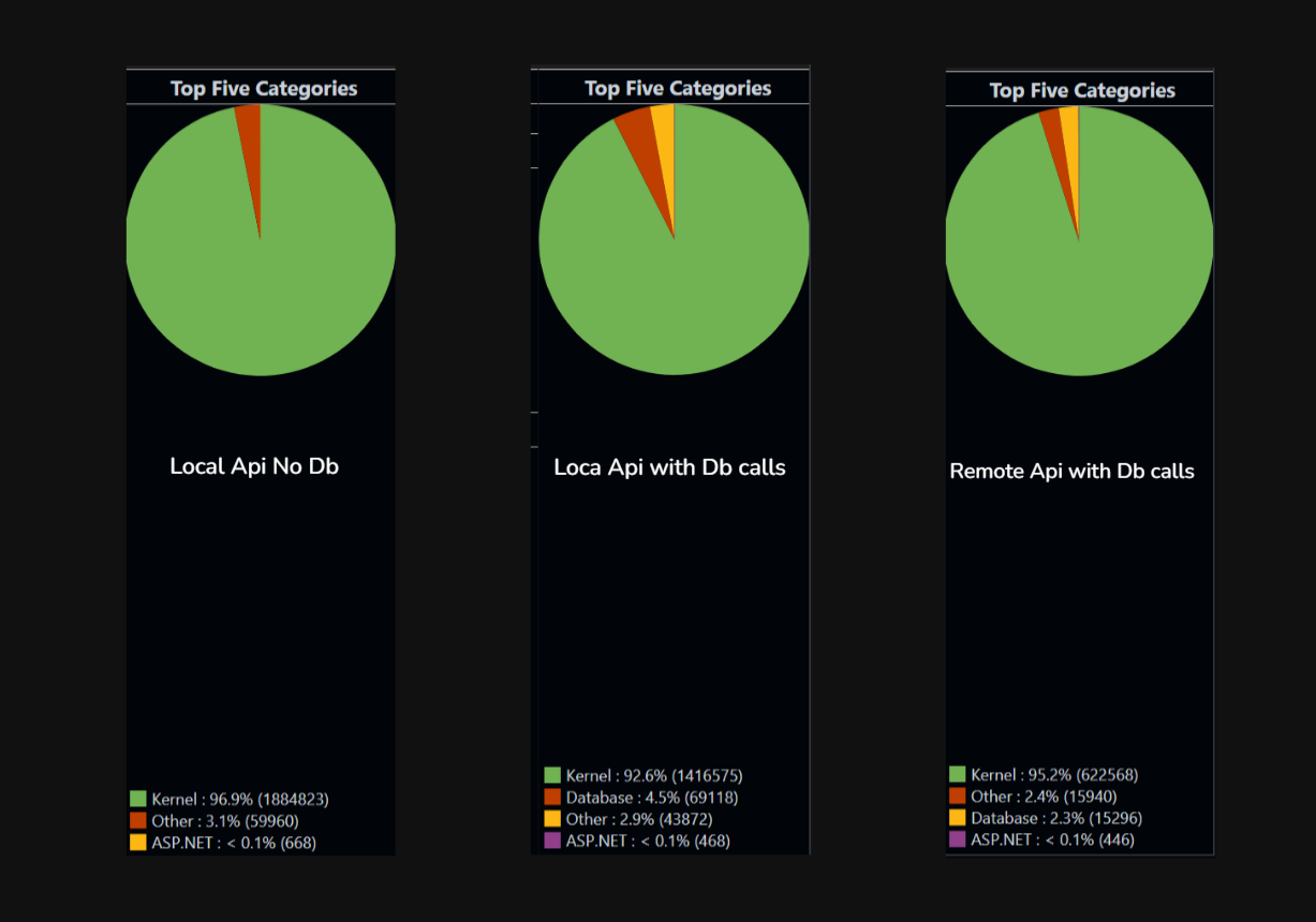
API isn’t doing much, the real work is at the kernel level. Serving incoming HTTP requests, establishing the TCP connection, reading bytes off the socket, putting in accept queue, writing the response, pushing bytes back out. That’s hundreds of syscalls just to move my HTTP traffic in and out.
Now let’s jump to the next layer. I’ll keep one rule throughout: p90 < 500ms. I know that’s generous, but this is a local machine and everything from server to client and database all are here.
Layer 3 : 1000 to 10000
Database connection pool now 300 connection max and now lets go to 5k users first
| Metric | This 5K (gradual ramp) |
|---|---|
| Throughput | 2,717 rps |
| Total requests | 2,608,544 |
| p50 latency | 460 ms |
| p95 latency | 4.45 s |
| p99 latency | 6.41 s |
| Max latency | 15.8 s |
| Avg latency | 1,100 ms |
| Failures | 0 |
Wi-Fi-bottlenecked system can do 2.7K rps with ~500ms median latency and a 5-second p95. That’s the real number.
Since we discovered network as our bottleneck at 5000 users where throughput was struck at 2717 requets/sec.
| Metric | 1K VUs (Wi-Fi) | 5K VUs (Wi-Fi) |
|---|---|---|
| Throughput | 4,584 rps | 2,717 rps ↓ |
| p50 | 123ms | 460ms |
| p95 | 251ms | 4.45s ↓↓ |
| Max | 5.7s | 15.8s |
We got 40% less throughput. This is the signature of a saturated system the Wi-Fi link couldn’t absorb 5K VUs, so packets queued, retransmitted, collided, and effective throughput collapsed
Here we are bringing client back to local device to eliminate that and see what else blocks our target to reach 10000 concurrent users.
Now we are going local client at 5000 virtual users.
Local client at 7000 virtual users.
| Test | VUs | Throughput | p50 | p95 | p99 | Max | Failures |
|---|---|---|---|---|---|---|---|
| DB local | 1,000 | 9,326 rps | 53ms | 113ms | 296ms | 15.7s | 55 |
| DB local | 5,000 | 14,906 rps | 172ms | 365ms | 527ms | 2.45s | 0 |
| DB local | 7,500 | 14,228 rps | 263ms | 505ms | 673ms | 2.18s | 0 |
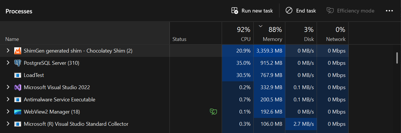
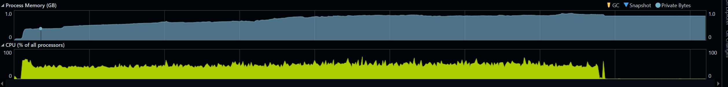
Snapshot of Task Manager at 5k virtual users
The system is now in a state where:
-
Connection pool is constantly saturated, every request waits for a connection
-
CPU is being shared between k6 (driving load), .NET app (handling requests), and Postgres (executing queries) on the same machine
-
k6 itself is probably using 4-6 GB of memory and significant CPU for 7500 VUs
-
No headroom left ,adding more load just creates queue depth, not more work The fact that throughput slightly decreased tells you all three contenders (k6, app, DB) are now fighting for resources. Each gets less than they would in isolation.
-
15K rps is the DB stack’s true ceiling on this hardware
-
5K VUs is the optimal load point peak throughput at lowest possible latency for my PC.
the most important thing across all these tests:
Adding more load to a saturated system makes it slower, not faster. The intuition that “more users = more throughput” only holds below the knee of the curve. Above it, throughput is flat or declining while latency explodes. Production systems hit this exact pattern during traffic spikes
| Test | VUs | Throughput | p50 | p95 | p99 |
|---|---|---|---|---|---|
| GetAge local | 1,000 | 28,807 rps | 19ms | 35ms | 50ms |
| GetAge local | 7,500 | 28,871 rps | 40ms | 160ms | 331ms |
| DB local | 5,000 | 14,906 rps | 172ms | 365ms | 527ms |
| DB local | 7,500 | 14,228 rps | 263ms | 505ms | 673ms |
This is the cleanest possible result that we have hit the server’s true CPU ceiling for this workload. With pure CPU work and no I/O wait, the server can do exactly ~29K rps and no more it doesn’t matter if we throw 1000 or 7500 VUs at it. The CPU is fully saturated either way.
The only difference between the two runs is latency: at 1K VUs, requests fly through (50ms p99); at 7.5K VUs, they queue (331ms p99). Same throughput, different waiting time.
HTTP keep-alive saves us from port exhaustion at this scale. Each VU keeps one TCP connection open and reuses it for thousands of requests, instead of opening a new connection per request. The 7500 VUs only need ~7500 ports, not 36 million.
How will we reach 10k and beyond
The first step is putting k6 on a separate machine, ideally connected via wired Ethernet rather than Wi-Fi. This single change eliminates the CPU contention we kept seeing in the local tests. k6, the .NET app, and Postgres all fighting for the same cores. With that contention gone, the same server hardware that capped at 14K rps would comfortably push past 22K rps, and 10K concurrent VUs becomes trivially achievable. The bottleneck stops being “this laptop is doing too much” and starts being something we can actually optimize.
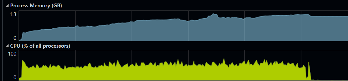
Past that point, the constraints shift to the layers we haven’t touched yet Postgres will need more memory to support a larger connection pool each connection costs 2 MB to 10 MB on the server side, so growing from 100 to 300 connections means another ~1 to 2GB just for backend processes, he .NET server will need more memory too, both for the thread pool growing under load and for the in-flight request/response buffers that pile up when concurrency rises.
Eventually we’ll hit ephemeral port exhaustion the OS only has ~28K ports available by default for outgoing connections, so a load generator opening short-lived connections will run out and start failing.
We can add Redis to bypass hot reads from db but again, more memory on same machine, redis if not configured will increase latency as well
All of this still lives on one server. We’re intentionally not touching distributed systems here, no horizontal scaling, no load balancer across multiple machines, no replicated database because the single-machine ceiling is already in the hundreds of thousands of requests per second once each layer is properly tuned, and most real applications with 1000s of users never need more than that. Distributed systems solve a fundamentally different problem (fault tolerance, geographic distribution, scale beyond one machine), and they introduce their own complexity that deserves its own discussion. For now, the takeaway is that a single well tuned server can handle far more than people assume and the path from 10K to 100K rps is just systematically removing the next bottleneck identified on the way, one layer at a time.
Thanks for reading.
Feel free to connect with me on (rahuldsoni2001@gmail.com)